
Register-transfer-level (RTL) development is widely known to be considerably more difficult than developing with more common high-level languages. The primary reason for this increased difficulty lies in the necessity for hardware expertise to craft efficient designs. However, even seasoned hardware engineers encounter distinct challenges that diverge sharply from those encountered in software development. These challenges stem from one issue that all hardware designers eventually come to realize: RTL code can be very weird.
In this article, we’ll explore an example of this weirdness, where semantically equivalent code synthesizes into markedly different circuits—sometimes selectively in certain tools, adding another layer of complexity. We’ll also investigate methods for identifying such issues and, in some cases, leveraging this weirdness for non-obvious optimizations.
Due to the common occurrence of RTL and FPGA weirdness, this article marks the first in an ongoing series where I will detail many of the unusual problems I’ve encountered throughout my career.
Example: multiple comparisons
Let’s examine a simple example involving a module that compares pairs of values. If all pairs are equal, the module outputs 1; otherwise, it outputs 0. Additionally, we will register both the input and output to analyze timing differences.
We’ll examine six different experiments, each implementing this behavior in a different way. As hinted by the article’s title, despite all six simulations having the same simulation behavior, we’ll encounter some weird results after synthesis.
Experiment 1:
module compare1 #(
    parameter int DATA_WIDTH = 16
) (
    input  logic                  clk,
    input  logic [DATA_WIDTH-1:0] a1, a2,
    input  logic [DATA_WIDTH-1:0] b1, b2,
    input  logic [DATA_WIDTH-1:0] c1, c2,
    input  logic [DATA_WIDTH-1:0] d1, d2,
    output logic                  eq
);
    logic [DATA_WIDTH-1:0] a1_r, a2_r;
    logic [DATA_WIDTH-1:0] b1_r, b2_r;
    logic [DATA_WIDTH-1:0] c1_r, c2_r;
    logic [DATA_WIDTH-1:0] d1_r, d2_r;

    always_ff @(posedge clk) begin
        // Register the inputs.
        a1_r <= a1; a2_r <= a2;
        b1_r <= b1; b2_r <= b2;
        c1_r <= c1; c2_r <= c2;
        d1_r <= d1; d2_r <= d2;

        // Compare the four pairs of inputs.
        if (a1_r == a2_r && b1_r == b2_r && c1_r == c2_r && d1_r == d2_r) begin
            eq <= 1'b1;
        end else begin
            eq <= 1'b0;
        end
    end
endmodule
This code first registers each input, then compares all four pairs of registers (a1_r with a2_r, b1_r with b2_r, etc.). If all pairs are equal the the module outputs 1 (via a register), otherwise it outputs 0.
Next, we’ll synthesize, place, and route this code in Vivado for an Ultrascale+ FPGA. The table below displays the lookup table (LUT) usage and the worst-case delays provided by the timing analyzer. Logic delay represents the sum of all “cells” along the longest path, which are FPGA primitives like LUTs, RAM, DSPs, etc. Net delay is the sum of all interconnect delays along the longest path, which may vary between experiments due to placement and routing differences. Total delay combines both logic and net delays.
| Experiment | LUTs | Logic Delay (ns) | Net Delay (ns) | Total Delay (ns) |
|---|---|---|---|---|
| compare1 | 27 | 0.479 | 0.390 | 0.880 |
Experiment 2:
One obvious limitation of the compare1 module is its hardcoded support for four pairs of inputs. To extend its functionality to handle pairs of any number of inputs, we will use two arrays: data_in1 and data_in2, with the size of each array array specified by the new NUM_INPUTS parameter. Here is the updated code:
module compare2 #(
    parameter int DATA_WIDTH = 16,
    parameter int NUM_INPUTS = 4
) (
    input  logic                  clk,
    input  logic [DATA_WIDTH-1:0] data_in1[NUM_INPUTS],
    input  logic [DATA_WIDTH-1:0] data_in2[NUM_INPUTS],
    output logic                  eq
);
    logic [DATA_WIDTH-1:0] data_in1_r[NUM_INPUTS];
    logic [DATA_WIDTH-1:0] data_in2_r[NUM_INPUTS];

    always @(posedge clk) begin
        logic temp;

        data_in1_r <= data_in1;
        data_in2_r <= data_in2;
        temp = 1'b1;

        for (int i = 0; i < NUM_INPUTS; i++) begin
            temp &= data_in1_r[i] == data_in2_r[i];
        end

        eq <= temp;
    end
endmodule
This code mimics the behavior of Experiment 1 but handles NUM_INPUTS comparisons by iterating through pairs and combining results using bitwise AND (&) operations. I do not recommend using this approach for actual implementation; rather, we are simply experimenting to understand how synthesis treats this behavior.
For this loop approach to work, the first iteration must bitwise AND the comparison result with a 1’b1. To achieve this, we declare a temporary logic signal, temp, initialized to 1’b1 before entering the loop. It’s important to note the use of a blocking assignment here; without it, this approach would not function correctly. Additionally, I’ve chosen to declare temp within the always block itself, which is unconventional but recommended in this scenario. This decision confines temp‘s scope to the always block, mitigating potential problems from blocking assignments on clock edges that extend beyond the block’s boundaries. While some guidelines prohibit the use of blocking assignments on clock edges altogether, I advocate for their cautious use, provided one fully comprehends their implications in synthesis.
Interestingly, if you’re familiar with VHDL, you might notice that my scoping of temp and the use of a blocking assignment mirror the semantics of a VHDL variable. This similarity is intentional. VHDL restricts the scope of variables to processes or blocks for a significant reason: it prevents race conditions that cause frequent problems in Verilog code.
Let’s now expand our results to see if the synthesized circuit matches the compare1 module:
| Experiment | LUTs | Logic Delay (ns) | Net Delay (ns) | Total Delay (ns) |
|---|---|---|---|---|
| compare1 | 27 | 0.479 | 0.390 | 0.880 |
| compare2 | 27 | 0.401 | 0.479 | 0.880 |
We’ve encountered some unexpected results. First, the good news: both compare1 and compare2 synthesize to identical circuits with 27 LUTs. What’s particularly weird (even to me) is that despite identical circuits, I anticipated identical logic delays. Each design’s longest path passes through three LUT6 primitives, so what accounts for the difference? To investigate, I examined the path report in the timing analyzer. Surprisingly, I found that the same type of primitive (e.g., LUT6) exhibits slight variations in delay due to placement. While it’s well-known that interconnect (net) delays vary with placement, I was surprised to observe discrepancies in logic delays for identical synthesized circuits. Curiously, both designs happen to share the exact same total delay.
Setting aside the peculiarities of the timing data, the key takeaway is that the compare1 and compare2 modules are indeed identical post-synthesis. Vivado simply manages their placement differently, resulting in timing discrepancies.
Experiment 3
You might have been confused why Experiment 2 used such complicated code. I’m hoping you might have wondered why we didn’t just compare the two input arrays. Good news! We can. Here’s the much simpler code:
module compare3 #(
    parameter int DATA_WIDTH = 16,
    parameter int NUM_INPUTS = 4
) (
    input  logic                  clk,
    input  logic [DATA_WIDTH-1:0] data_in1[NUM_INPUTS],
    input  logic [DATA_WIDTH-1:0] data_in2[NUM_INPUTS],
    output logic                  eq
);
    logic [DATA_WIDTH-1:0] data_in1_r[NUM_INPUTS];
    logic [DATA_WIDTH-1:0] data_in2_r[NUM_INPUTS];

    always @(posedge clk) begin
        data_in1_r <= data_in1;
        data_in2_r <= data_in2;
        eq         <= data_in1_r == data_in2_r;
    end
endmodule
This code is clearly more concise and readable than Experiment 2. However, let’s verify that it synthesizes to the same circuit:
| Experiment | LUTs | Logic Delay (ns) | Net Delay (ns) | Total Delay (ns) |
|---|---|---|---|---|
| compare1 | 27 | 0.479 | 0.390 | 0.880 |
| compare2 | 27 | 0.401 | 0.479 | 0.880 |
| compare3 | 27 | 0.401 | 0.479 | 0.880 |
Good news again: compare3 is identical to compare2, both in synthesis and in timing analysis. Experiments 1-3 all result in the same synthesized circuit.
Experiment 4:
Let’s revisit Experiment 1 and again restrict ourselves to four pairs of inputs. In the compare1 module, we individually compared all four pairs of inputs and then combined those results using bitwise AND operations. Let’s attempt a more concise approach. Instead of performing four separate comparisons, we can concatenate all the {a-d}1 inputs together, concatenate the {a-d}2 inputs together, and then perform a single, wider comparison of all pairs at once. Here’s the corresponding code:
module compare4 #(
    parameter int DATA_WIDTH = 16
) (
    input  logic                  clk,
    input  logic [DATA_WIDTH-1:0] data_in1[4],
    input  logic [DATA_WIDTH-1:0] data_in2[4],
    output logic                  eq
);
    logic [DATA_WIDTH-1:0] data_in1_r[4];
    logic [DATA_WIDTH-1:0] data_in2_r[4];

    always_ff @(posedge clk) begin
        data_in1_r <= data_in1;
        data_in2_r <= data_in2;
        eq         <= {data_in1_r[0], data_in1_r[1], data_in1_r[2], data_in1_r[3]} ==
                      {data_in2_r[0], data_in2_r[1], data_in2_r[2], data_in2_r[3]};
    end
endmodule
As expected, this code simulates identically to the previous three experiments. However, let’s take a look at the synthesis results:
| Experiment | LUTs | Logic Delay (ns) | Net Delay (ns) | Total Delay (ns) |
|---|---|---|---|---|
| compare1 | 27 | 0.479 | 0.390 | 0.880 |
| compare2 | 27 | 0.401 | 0.479 | 0.880 |
| compare3 | 27 | 0.401 | 0.479 | 0.880 |
| compare4 | 22 | 0.505 | 0.350 | 0.855 |
We’ve encountered another weird result. Experiment 4 uses fewer LUTs and has lower total delay than Experiments 1-3. I’ll explain the reasons for this later, but first, let’s examine some other experiments to gain further insights.
Experiment 5:
The concatenation approach in Experiment 4 suggests a similar test using structs to encapsulate all the data, thereby implicitly handling the concatenation. Here is the updated code:
package compare_pkg;
    localparam int DATA_WIDTH = 16;
    typedef struct packed {
        logic [DATA_WIDTH-1:0] in0;
        logic [DATA_WIDTH-1:0] in1;
        logic [DATA_WIDTH-1:0] in2;
        logic [DATA_WIDTH-1:0] in3;
    } CompareStruct;
endpackage

module compare5
    import compare_pkg::*;
(
    input  logic                      clk,
    input  compare_pkg::CompareStruct data_in1,
    input  compare_pkg::CompareStruct data_in2,
    output logic                      eq
);
    compare_pkg::CompareStruct data_in1_r;
    compare_pkg::CompareStruct data_in2_r;

    always_ff @(posedge clk) begin
        data_in1_r <= data_in1;
        data_in2_r <= data_in2;
        eq         <= data_in1_r == data_in2_r;
    end
endmodule
Let’s now synthesize this and update our results:
| Experiment | LUTs | Logic Delay (ns) | Net Delay (ns) | Total Delay (ns) |
|---|---|---|---|---|
| compare1 | 27 | 0.479 | 0.390 | 0.880 |
| compare2 | 27 | 0.401 | 0.479 | 0.880 |
| compare3 | 27 | 0.401 | 0.479 | 0.880 |
| compare4 | 22 | 0.505 | 0.350 | 0.855 |
| compare5 | 22 | 0.505 | 0.350 | 0.855 |
Interestingly, Experiment 5 mirrors Experiment 4, using fewer resources and achieving faster clock frequencies than Experiments 1-3. We’ll revisit this observation later.
Experiment 6:
Let’s conduct one more experiment. The drawback of Experiments 4 and 5 is that they are hardcoded for four inputs. Ideally, we would find an approach that achieves the same results but is fully parameterized. Let’s revisit Experiment 3, where we compared two unpacked, parameterized arrays. In this experiment, we’ll simply update the code to use packed arrays and observe the outcome:
module compare6 #(
    parameter int DATA_WIDTH = 16,
    parameter int NUM_INPUTS = 4
) (
    input  logic                                  clk,
    input  logic [DATA_WIDTH-1:0][NUM_INPUTS-1:0] data_in1,
    input  logic [DATA_WIDTH-1:0][NUM_INPUTS-1:0] data_in2,
    output logic                                  eq
);
    logic [DATA_WIDTH-1:0][NUM_INPUTS-1:0] data_in1_r;
    logic [DATA_WIDTH-1:0][NUM_INPUTS-1:0] data_in2_r;

    always @(posedge clk) begin
        data_in1_r <= data_in1;
        data_in2_r <= data_in2;
        eq         <= data_in1_r == data_in2_r;
    end
endmodule
Finally, let’s complete our results table:
| Experiment | LUTs | Logic Delay (ns) | Net Delay (ns) | Total Delay (ns) |
|---|---|---|---|---|
| compare1 | 27 | 0.479 | 0.390 | .880 |
| compare2 | 27 | 0.401 | 0.479 | .880 |
| compare3 | 27 | 0.401 | 0.479 | .880 |
| compare4 | 22 | 0.505 | 0.350 | 0.855 |
| compare5 | 22 | 0.505 | 0.350 | 0.855 |
| compare6 | 22 | 0.390 | 0.434 | 0.824 |
The compare6 module yields different results from the compare3 module! How is this possible? The modules are identical except for the use of packed versus unpacked arrays, which theoretically should not affect synthesis. These results might suggest that packed arrays are inherently better for synthesis, but this is not generally the case. We need to continue investigating to understand how Vivado is handling each of these experiments.
Synthesis Analysis
We will now examine the lower-level details of each synthesized example to identify any patterns that might explain Vivado’s behavior. This type of analysis is a valuable exercise for any code examples. Performing these experiments will deepen your understanding of synthesis and help you recognize the peculiar behaviors of different tools.
The first step I always take after designing any module is to examine the schematic of the elaborated design to ensure it matches my expectations. Below is the schematic for Experiments 1-3 (note that the experiments’ nets have different names but the same structure):
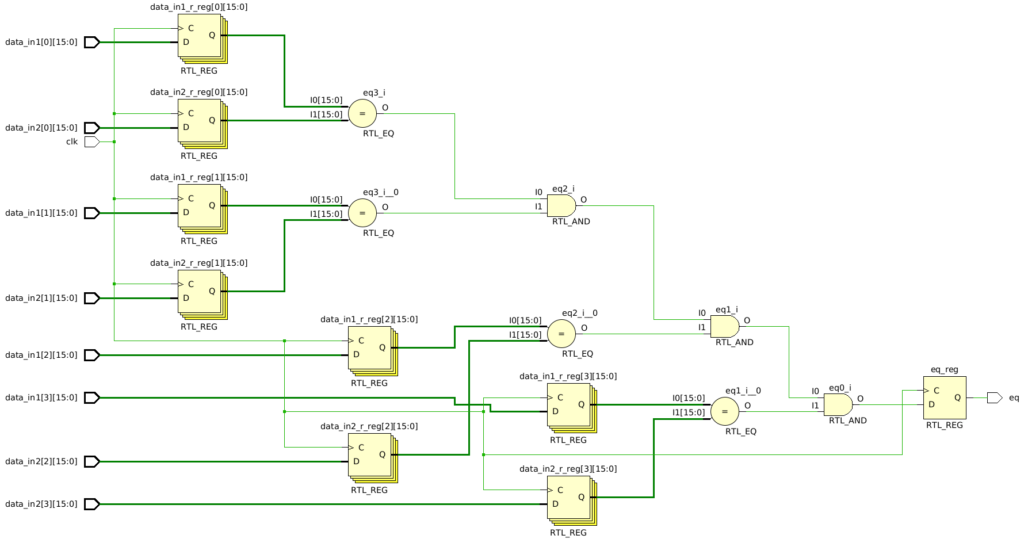
This schematic appears to make sense. The inputs are all registered, and we observe four separate comparisons that are sequentially ANDed together before being stored in an output register. Based solely on this schematic, there doesn’t seem to be anything unusual.
Let’s now examine the schematic for Experiments 4-6 (again, they have different net names, but identical structure):
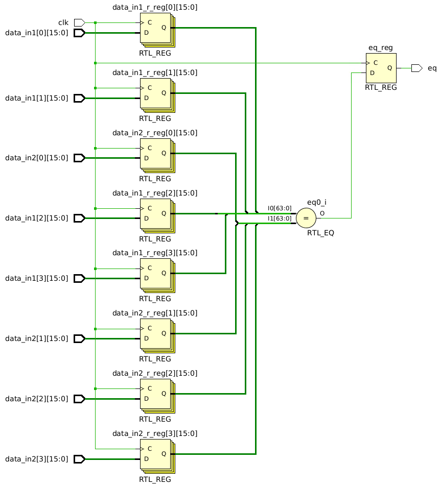
An obvious difference in this schematic is that instead of four separate comparisons and multiple AND gates, there is a single, wider comparison. Should this difference matter? Logically, there is no difference between ANDing multiple comparisons of pairs of inputs and comparing two sets of concatenated inputs, so we would expect the synthesized circuits to be identical.
We need to keep looking, so instead of the elaborated schematic, let’s examine the post-synthesis schematic. Below is the schematic for Experiments 1-3:
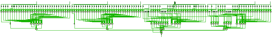
The schematic is too small to discern the details clearly, but take note of the visual pattern; we’ll analyze it in detail shortly.
Next, here is the schematic for Experiments 4-6:
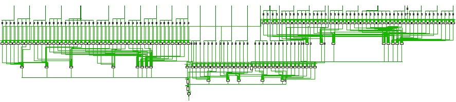
Clearly, there is a difference in the synthesized circuits. What’s going on here?
If you open these examples in Vivado, synthesize them, and then view the schematic, you should be able to zoom in and observe some important details. Since I can’t display it visually here, I’ll summarize the key differences. In Experiments 1-3, the inputs pass through up to three LUT6 primitives before reaching the output register, as shown by the timing analyzer:
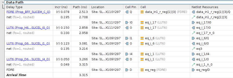
The total logic delay for this path is 0.401 ns, with an interconnect delay of 0.479 ns, resulting in a total delay of 0.880 ns. This corresponds to the results observed in Experiment 3.
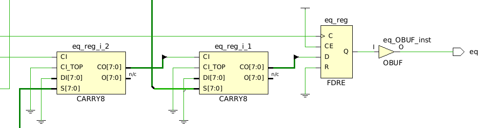
In Experiments 4-6, the inputs pass through a single LUT6 primitive before proceeding through up to three CARRY8 primitives. Here’s a snippet of the post-synthesis schematic:
Here is the longest path from the timing analyzer for Experiment 6:
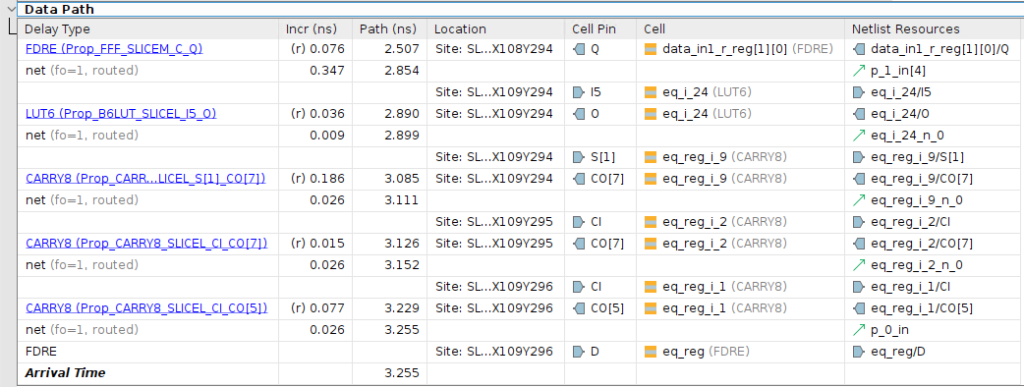
This path has a total logic delay of 0.39 ns and an interconnect delay of 0.434 ns, both of which are smaller than those in Experiment 3. The most significant improvement is the reduced interconnect delay between the CARRY8 primitives (0.026 ns), compared to a minimum of 0.1 ns between the LUT6 primitives in Experiment 3. CARRY8 primitives benefit from dedicated, hardened interconnect, while LUT6 primitives rely on the slower, reconfigurable interconnect.
Explanation of Differences
We now have strong evidence about which approach works better in Vivado, but we still need to understand why. The difference arises from Vivado’s inability to recognize that ANDing a series of comparisons is equivalent to performing a single, wider comparison. This issue becomes apparent when examining the elaboration schematics shown earlier. In Experiments 1-3, we explicitly see four comparisons followed by a sequence of AND gates. It is these AND gates that contribute to the problem. In contrast, Experiments 4-6 involve only a single comparison.
Why is a single comparison more efficient than performing four smaller comparisons followed by several AND gates? Generally, it shouldn’t be. The observed difference arises from technology mapping. Vivado has optimized wide reduction operations, such as comparisons, for technology mapping. In this case, technology mapping maps the wide comparison reduction onto CARRY8 primitives, which are specifically designed for such operations. The documentation for the CARRY8 even mentions its use for wide comparators.
Why, then, can’t Vivado simply convert Experiments 1-3 into a single wide comparison? Technically, it could, but with the massive number of possible conversions between sequences of operations, it is inevitable that tools are going to miss some of these optimizations. Out of curiosity, I repeated these experiments in Intel Quartus Prime Pro, which was able to perform the conversion to a single comparator and synthesize identical circuits for all the experiments. The timing was even identical, which highlights a quirk of Vivado that will be the subject of a future article.
Finally, we need to address the peculiar difference between Experiment 3 and Experiment 6, where the only change was switching from unpacked to packed input arrays. While it’s difficult to pinpoint the exact cause, it seems that Vivado may implicitly convert a comparison of unpacked arrays into a form similar to Experiment 2, where each comparison is ANDed with the results of previous iterations. In contrast, Vivado appears to handle packed arrays by directly comparing the bits, similar to the manual concatenation or struct approach we used. This result does not imply that packed arrays are inherently better than unpacked arrays; rather, it highlights another quirk in Vivado’s implementation. Ideally, Vivado would standardize the handling of different array types to ensure consistent results. Until then, this difference represents an opportunity to exploit tool-specific behavior for more efficient design.
Conclusions
We’ve gained several insights from this study. First, we discovered a useful Vivado-specific optimization for comparing multiple values. However, the primary takeaway is not just this specific optimization but the methodology we used to identify the unusual behavior. We started with the expectation that similar simulated behaviors should synthesize identically, but this wasn’t the case. By examining the low-level synthesis details for each example, we uncovered two key findings: Vivado can optimize wide comparisons using CARRY8 primitives instead of just LUTs, and Vivado cannot always convert sequences of comparisons into a single wide comparison. While the specifics of this example might not make you a professional RTL designer, the process we followed to uncover this optimization will. Applying this approach to various modules throughout your career will help you navigate the peculiarities of RTL design and leverage them to create highly efficient designs.